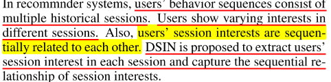
写在前面
DSIN 全称是 Deep Session Interest Network (深度会话兴趣网络), 重点在这个 Session 上,这个是在 DIEN 的基础上又进行的一次演化,这个模型的改进出发点依然是如何通过用户的历史点击行为,从里面更好的提取用户的兴趣以及兴趣的演化过程,这个模型就是从 user 历史行为信息挖掘方向上进行演化的。而提出的动机呢? 就是作者发现用户的行为序列的组成单位,其实应该是会话 (按照用户的点击时间划分开的一段行为),每个会话里面的点击行为呢? 会高度相似,而会话与会话之间的行为,就不是那么相似了,但是像 DIN,DIEN 这两个模型,DIN 的话,是直接忽略了行为之间的序列关系,使得对用户的兴趣建模或者演化不是很充分,而 DIEN 的话改进了 DIN 的序列关系的忽略缺点,但是忽视了行为序列的本质组成结构。所以阿里提出的 DSIN 模型就是从行为序列的组成结构会话的角度去进行用户兴趣的提取和演化过程的学习,在这个过程中用到了一些新的结构,比如 Transformer 中的多头注意力,比如双向 LSTM 结构,再比如前面的局部 Attention 结构。
DSIN 模型的理论以及论文细节
DSIN 的简介与进化动机
DSIN 模型全称叫做 Deep Session Interest Network, 这个是阿里在 2019 年继 DIEN 之后的一个新模型, 这个模型依然是研究如何更好的从用户的历史行为中捕捉到用户的动态兴趣演化规律。而这个模型的改进动机呢? 就是作者认为之前的序列模型,比如 DIEN 等,忽视了序列的本质结构其实是由会话组成的:
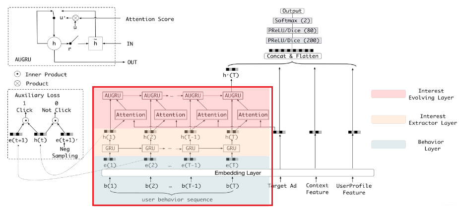
这是个啥意思呢? 其实举个例子就非常容易明白 DIEN 存在的问题了 (DIN 这里就不说了,这个存在的问题在 DIEN 那里说的挺详细了,这里看看 DIEN 有啥问题),上一篇文章中我们说 DIEN 为了能够更好的利用用户的历史行为信息,把序列模型引进了推荐系统,用来学习用户历史行为之间的关系, 用兴趣提取层来学习各个历史行为之间的关系,而为了更有针对性的模拟与目标广告相关的兴趣进化路径,又在兴趣提取层后面加了注意力机制和兴趣进化层网络。这样理论上就感觉挺完美的了啊。这里依然是把 DIEN 拿过来,也方便和后面的 DSIN 对比:
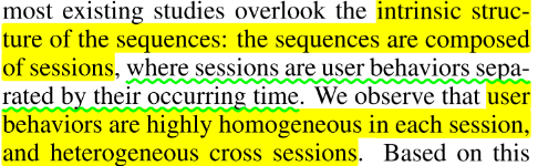
但这个模型存在个啥问题呢? 就是只关注了如何去改进网络,而忽略了用户历史行为序列本身的特点, 其实我们仔细想想的话,用户过去可能有很多历史点击行为,比如 [item3, item45, item69, item21, .....] , 这个按照用户的点击时间排好序了,既然我们说用户的兴趣是非常广泛且多变的,那么这一大串序列的商品中,往往出现的一个规律就是在比较短的时间间隔内的商品往往会很相似,时间间隔长了之后,商品之间就会出现很大的差别,这个是很容易理解的,一个用户在半个小时之内的浏览点击的几个商品的相似度和一个用户上午点击和晚上点击的商品的相似度很可能是不一样的。这其实就是作者说的 homogeneous 和 heterogeneous 。而 DIEN 模型呢? 它并没有考虑这个问题,而是会直接把这一大串行为序列放入 GRU 让它自己去学 (当然我们其实可以人工考虑这个问题,然后如果发现序列很长的话我们也可以分成多个样本哈,当然这里不考虑这个问题),如果一大串序列一块让 GRU 学习的话,往往用户的行为快速改变和突然终止的序列会有很多噪声点,不利于模型的学习。
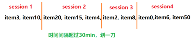
所以,作者这里就是从序列本身的特点出发, 把一个用户的行为序列分成了多个会话,所谓会话,其实就是按照时间间隔把序列分段,每一段的商品列表就是一个会话,那这时候,会话里面每个商品之间的相似度就比较大了,而会话与会话之间商品相似度就可能比较小。作者这里给了个例子:
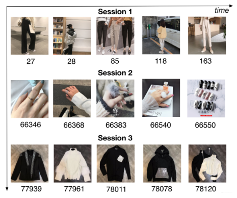
这是某个用户过去的历史点击行为,然后按照 30 分钟的时间间隔进行的分段,分成了 3 段。这里就一下子看出上面说的那些是啥意思了吧。就像这个女生,前 30 分钟在看裤子,再过 30 分钟又停留在了化妆品,又过 30 分钟,又看衣服。这种现象是非常普遍的啊,反映了一个用户通常在某个会话里面会有非常单一的兴趣但是当过一段时间之后,兴趣就会突然的改变。这个时候如果再统一的考虑所有行为就不合理了呀。这其实也是 DSIN 改进的动机了, DSIN,这次的关键就是在 S 上。
那它要怎么改呢? 如果是我们的话应该怎么改呢? 那一定会说,这个简单啊,不是说 DIEN 没考虑序列本身的特点吗? 既然我们发现了上面用户点击行为的这种会话规律,那么我们把序列进行分段,然后再用 DIEN 不就完事了? 哈哈, 那当然可以呀, 如果想用 DIEN 的话确实可以这么玩, 但那样就没有新模型了啊,那不还是 DIEN? 这样的改进思路是没法发顶会的哟哈哈。 下面分析下人家是怎么改进的。
简单的说是用了四步,这个也是 DSIN 模型的整体逻辑:
首先, 分段这个是必须的了吧,也就是在用户行为序列输入到模型之前,要按照固定的时间间隔 (比如 30 分钟) 给他分开段,每一段里面的商品序列称为一个会话 Session。 这个叫做会话划分层
然后呢,就是学习商品时间的依赖关系或者序列关系,由于上面把一个整的行为序列划分成了多段,那么在这里就是每一段的商品时间的序列关系要进行学习,当然我们说可以用 GRU, 不过这里作者用了多头的注意力机制,这个东西是在多个角度研究一个会话里面各个商品的关联关系, 相比 GRU 来讲,没有啥梯度消失,并且可以并行计算,比 GRU 可强大多了。这个叫做会话兴趣提取层
上面研究了会话内各个商品之间的关联关系,接下来就是研究会话与会话之间的关系了,虽然我们说各个会话之间的关联性貌似不太大,但是可别忘了会话可是能够表示一段时间内用户兴趣的, 所以研究会话与会话的关系其实就是在学习用户兴趣的演化规律,这里用了双向的 LSTM,不仅看从现在到未来的兴趣演化,还能学习未来到现在的变化规律, 这个叫做会话交互层。
既然会话内各个商品之间的关系学到了,会话与会话之间的关系学到了,然后呢? 当然也是针对性的模拟与目标广告相关的兴趣进化路径了, 所以后面是会话兴趣局部激活层, 这个就是注意力机制, 每次关注与当前商品更相关的兴趣。
所以,我们细品一下,其实 DSIN 和思路和 DIEN 的思路是差不多的,无非就是用了一些新的结构,这样,我们就从宏观上感受了一波这个模型。接下来,研究架构细节了。 看看上面那几块到底是怎么玩的。
DSIN 的架构剖析
这里在说 DSIN 之前,作者也是又复习了一下 base model 模型架构,这里我就不整理了,其实是和 DIEN 那里一模一样的,具体的可以参考我上一篇文章。直接看 DSIN 的架构:
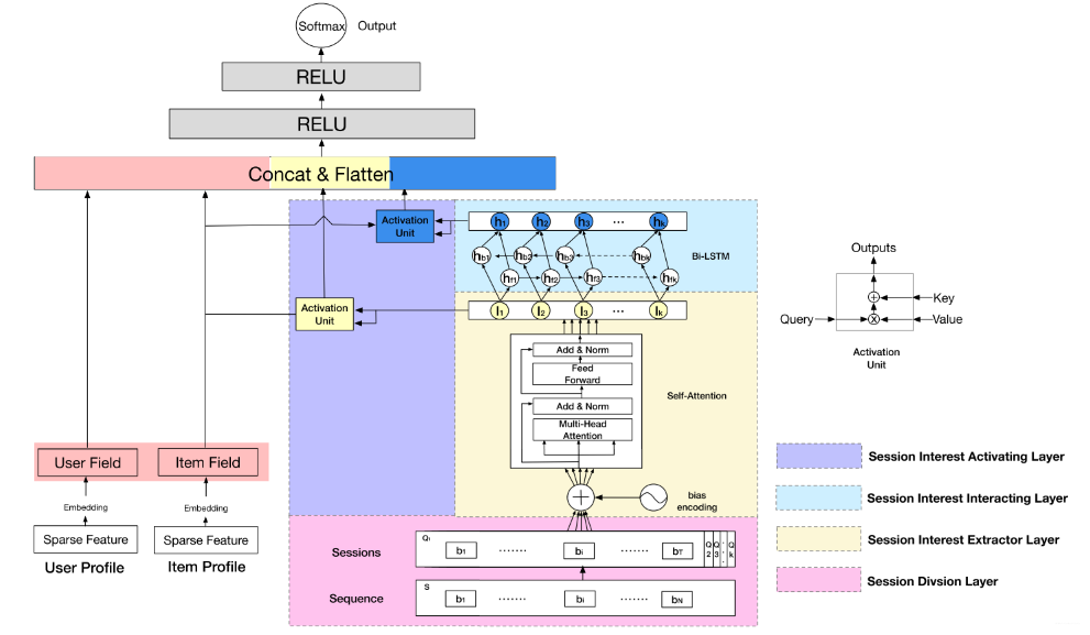
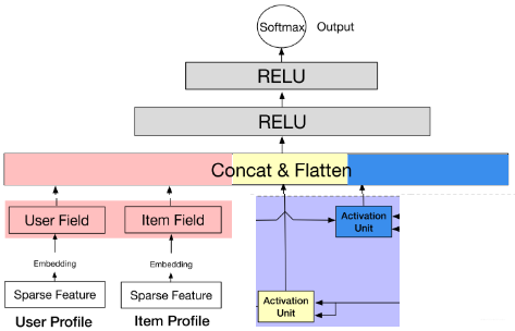
这个模型第一印象又是挺吓人的。核心的就是上面剖析的那四块,这里也分别用不同颜色表示出来了。也及时右边的那几块,左边的那两块还是我们之前的套路,用户特征和商品特征的串联。这里主要研究右边那四块,作者在这里又强调了下 DSIN 的两个目的,而这两个目的就对应着本模型最核心的两个层 (会话兴趣提取层和会话交互层):
Session Division Layer
这一层是将用户的行为序列进行切分,首先将用户的点击行为按照时间排序,判断两个行为之间的时间间隔,如果前后间隔大于 30min,就进行切分 (划一刀), 当然 30min 不是定死的,具体跟着自己的业务场景来。
划分完了之后,我们就把一个行为序列
Session Interest Extractor Layer
这个层是学习每个会话中各个行为之间的关系,之前也分析过,在同一个会话中的各个商品的相关性是非常大的。此外,作者这里还提到,用户的随意的那种点击行为会偏离用户当前会话兴趣的表达,所以为了捕获同一会话中行为之间的内在关系,同时降低这些不相关行为的影响,这里采用了 multi-head self-attention。关于这个东西, 这里不会详细整理,可以参考我之前的文章。这里只给出两个最核心关键的图,有了这两个图,这里的知识就非常容易理解了哈哈。
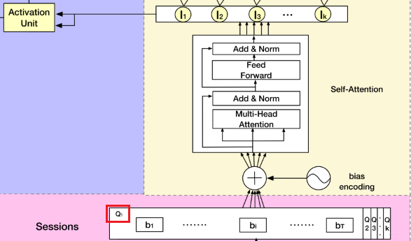
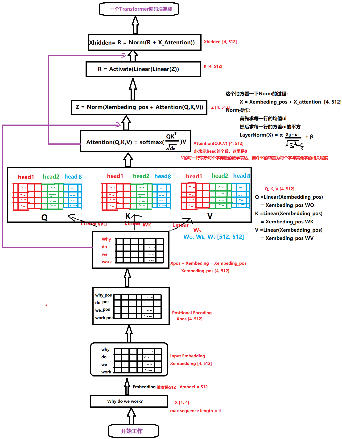
第一个,就是 Transformer 的编码器的一小块:
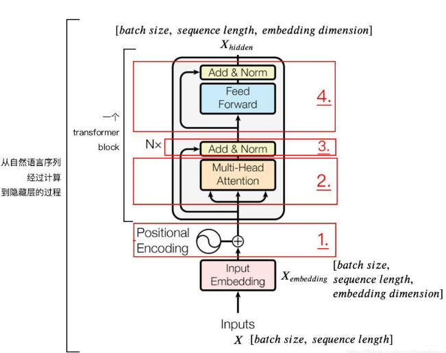
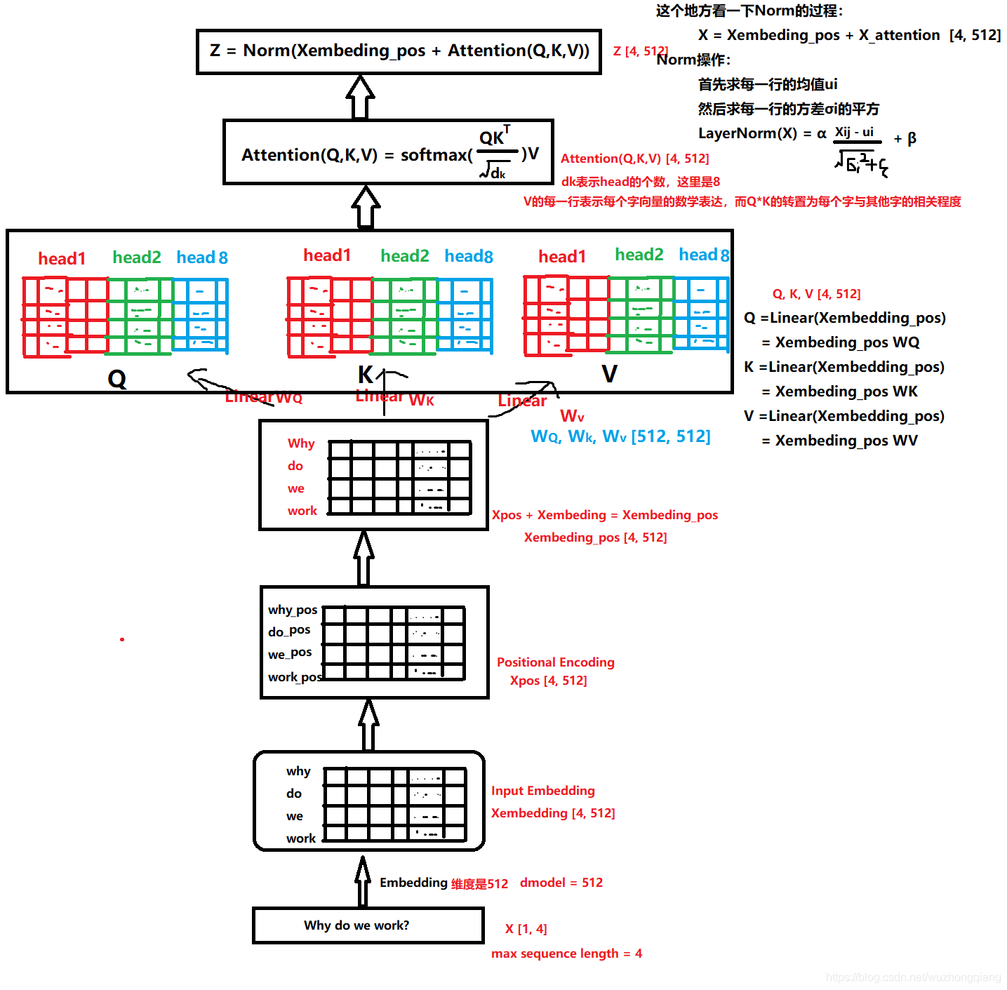
拿过来是为了更好的对比,看 DSIN 的结构的第二层,其实就是这个东西。 而这个东西的整体的计算过程,我在之前的文章中剖析好了:
有了上面这两张图,在解释这里就非常好说了。
这一块其实是分两步的,第一步叫做位置编码,而第二步就是 self-attention 计算关联。 同样,DSIN 中也是这两步,只不过第一步里面的位置编码,作者在这里做了点改进,称为 Bias Encoding。先看看这个是怎么做的。
这里先解释下为啥要进行位置编码或者 Bias Encoding, 这是因为我们说 self-attention 机制是要去学习会话里面各个商品之间的关系的, 而商品我们知道是一个按照时间排好的小序列,由于后面的 self-attention 并没有循环神经网络的迭代运算,所以我们必须提供每个字的位置信息给后面的 self-attention,这样后面 self-attention 的输出结果才能蕴含商品之间的顺序信息。
在 Transformer 中,对输入的序列会进行 Positional Encoding。Positional Encoding 对序列中每个物品,以及每个物品对应的 Embedding 的每个位置,进行了处理,如下:
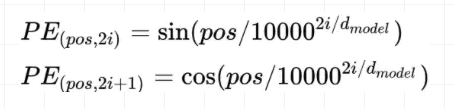
上式中
而这里,作者并不是用的这种方式,这是因为在这里还需要考虑各个会话之间的位置信息,毕竟这里是多个会话,并且各个会话之间也是有位置顺序的呀,所以还需要对每个会话添加一个 Positional Encoding, 在 DSIN 中,这种对位置的处理,称为 Bias Encoding。
于是乎作者在这里提出了个
所以
这个
接下来,就是每个会话的序列都通过 Transformer 进行处理:
一定要注意,这里说的是每个会话,这里我特意把下面的
首先
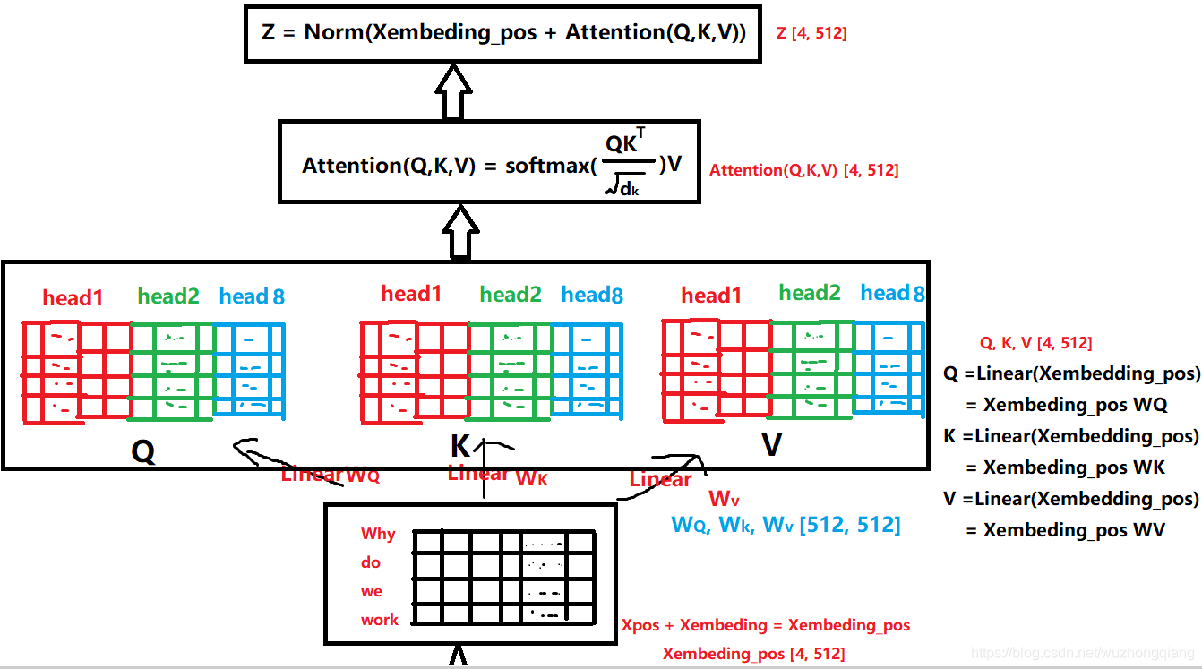
这里在拿过更细的个图来解释,首先这个
拿一个 head 来举例子:
我们看看这个在表示啥意思:
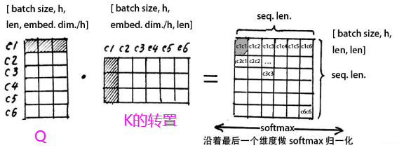
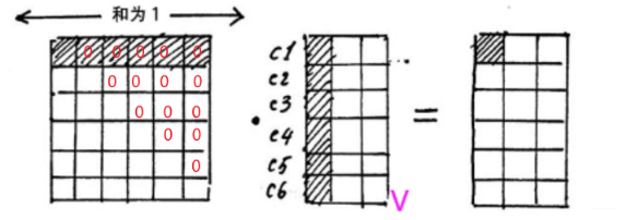
假设当前会话有 6 个物品,embedding 的维度是 3 的话,那么会看到这里一成,得到的结果中的每一行其实表示的是当前商品与其他商品之间的一个相似性大小 (embedding 内积的形式算的相似)。而沿着最后一个维度 softmax 归一化之后,得到的是个权重值。这是不是又想起我们的注意力机制来的啊,这个就叫做注意力矩阵,我们看看乘以 V 会是个啥
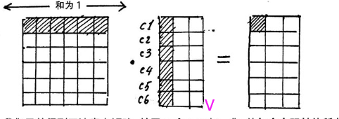
这时候,我们从注意力矩阵取出一行(和为 1),然后依次点乘 V 的列,因为矩阵 V 的每一行代表着每一个字向量的数学表达,这样操作,得到的正是注意力权重进行数学表达的加权线性组合,从而使每个物品向量都含有当前序列的所有物品向量的信息。而多头,不过是含有多个角度的信息罢了,这就是 Self-attention 的魔力了。
好了, 下面再看论文里面的描述就非常舒服了,如果令
这里是某一个头的计算过程, 这里的
这个是 self-attention 的输出再过一个全连接网络得到的。如果是用残差网络的话,最后的结果依然是个
即这个
不同点就是这里用了两个 transformer 块,开始用的是 bias 编码。
接下来就是不同的会话都走这样的一个 Transformer 网络,就会得到一个
- 这
个会话是走同一个 Transformer 网络的,也就是在自注意力机制中不同的会话之间权重共享 - 最后得到的这个矩阵,
这个维度上是有时间先后关系的,这为后面用 LSTM 学习这各个会话之间的兴趣向量奠定了基础。
Session Interest Interacting Layer
感觉这篇文章最难的地方在上面这块,所以我用了些篇幅,而下面这些就好说了,因为和之前的东西对上了又。 首先这个会话兴趣交互层

作者这里就是想通过一个双向的 LSTM 来学习下会话兴趣之间的关系, 从而增加用户兴趣的丰富度,或许还能学习到演化规律。
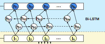
双向的 LSTM 这个,这里就不介绍了,关于 LSTM 之前我也总结过了,无非双向的话,就是先从头到尾计算,在从尾到头回来。所以这里每个时刻隐藏状态的输出计算公式为:
这是一个
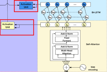
Session Interest Activating Layer
用户的会话兴趣与目标物品越相近,那么应该赋予更大的权重,这里依然使用注意力机制来刻画这种相关性,根据结构图也能看出,这里是用了两波注意力计算:
由于这里的这种局部 Attention 机制,DIN 和 DIEN 里都见识过了, 这里就不详细解释了, 简单看下公式就可以啦。
- 会话兴趣提取层
这里
这里
Output Layer
这个就很简单了,上面的用户行为特征, 物品行为特征以及求出的会话兴趣特征进行拼接,然后过一个 DNN 网络,就可以得到输出了。
损失这里依然用的交叉熵损失:
这里的
到这里 DSIN 模型就解释完毕了。
论文的其他细节
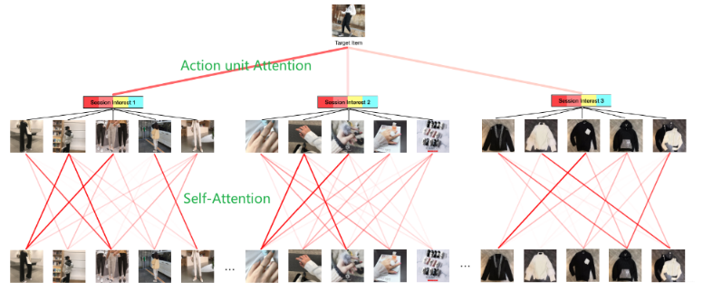
这里的其他细节,后面就是实验部分了,用的数据集是一个广告数据集一个推荐数据集, 对比了几个比较经典的模型 Youtubetnet, W&D, DIN, DIEN, 用了 RNN 的 DIN 等。并做了一波消融实验,验证了偏置编码的有效性, 会话兴趣抽取层和会话交互兴趣抽取层的有效性。 最后可视化的 self-attention 和 Action Unit 的图比较有意思:
好了,下面就是 DSIN 的代码细节了。
DSIN 的代码复现细节
下面就是 DSIN 的代码部分,这里我依然是借鉴了 Deepctr 进行的简化版本的复现, 这次复现代码会非常多,因为想借着这个机会学习一波 Transformer,具体的还是参考我后面的 GitHub。 下面开始:
数据处理
首先, 这里使用的数据集还是 movielens 数据集,延续的 DIEN 那里的,没来得及尝试其他,这里说下数据处理部分和 DIEN 不一样的地方。最大的区别就是这里的用户历史行为上的处理, 之前的是一个历史行为序列列表,这里得需要把这个列表分解成几个会话的形式, 由于每个用户的会话还不一定一样长,所以这里还需要进行填充。具体的数据格式如下:
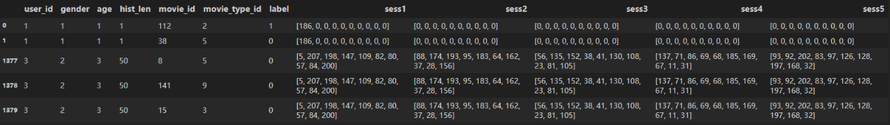
就是把之前的 hist_id 序列改成了 5 个 session。其他的特征那里没有变化。 而特征封装那里,需要把这 5 个会话封装起来,同时还得记录每个用户的有效会话个数以及每个会话里面商品的有效个数, 这个在后面计算里面是有用的,因为目前是 padding 成了一样长,后面要根据这个个数进行 mask, 所以这里有两波 mask 要做
feature_columns = [SparseFeat('user_id', max(samples_data["user_id"])+1, embedding_dim=8),
                    SparseFeat('gender', max(samples_data["gender"])+1, embedding_dim=8),
                    SparseFeat('age', max(samples_data["age"])+1, embedding_dim=8),
                    SparseFeat('movie_id', max(samples_data["movie_id"])+1, embedding_dim=8),
                    SparseFeat('movie_type_id', max(samples_data["movie_type_id"])+1, embedding_dim=8),
                    DenseFeat('hist_len', 1)]

feature_columns += [VarLenSparseFeat('sess1', vocabulary_size=max(samples_data["movie_id"])+1, embedding_dim=8, maxlen=10, length_name='seq_length1'),
                    VarLenSparseFeat('sess2', vocabulary_size=max(samples_data["movie_id"])+1, embedding_dim=8, maxlen=10, length_name='seq_length2'),
                    VarLenSparseFeat('sess3', vocabulary_size=max(samples_data["movie_id"])+1, embedding_dim=8, maxlen=10, length_name='seq_length3'),
                    VarLenSparseFeat('sess4', vocabulary_size=max(samples_data["movie_id"])+1, embedding_dim=8, maxlen=10, length_name='seq_length4'),
                    VarLenSparseFeat('sess5', vocabulary_size=max(samples_data["movie_id"])+1, embedding_dim=8, maxlen=10, length_name='seq_length5'),
                   ]
feature_columns += ['sess_length']
封装代码变成了上面这个样子, 之所以放这里, 我是想说明一个问题,也是我这次才刚刚发觉的,就是这块封装特征的代码是用于建立模型用的, 也就是不用管有没有数据集,只要基于这个 feature_columns 就能把模型建立出来。 而这里面有几个重要的细节要梳理下:
- 上面的那一块特征是常规的离散和连续特征,封装起来即可,这个会对应的建立 Input 层接收后面的数据输入
- 第二块的变长离散特征, 注意后面的
seq_length,这个东西的作用是标记每个用户在每个会话里面有效商品的真实长度,所以这 5 个会话建 Input 层的时候,不仅给前面的 sess 建立 Input,还会给 length_name 建立 Input 层来接收每个用户每个会话里面商品的真实长度信息, 这样在后面创建 mask 的时候才有效。也就是没有具体数据之前网络就能创建 mask 信息才行。这个我是遇到了坑的,之前又忽略了这个seq_length, 想着直接用上面的真实数据算出长度来给网络不就行? 其实不行,因为我们算出来的长度 mask 给网络的时候,那个样本数已经确定了,这时候会出 bug 的到后面。 因为真实训练的时候,batch_size 是我们自己指定。并且这个思路的话是网络依赖于数据才能建立出来,显然是不合理的。所以一定要切记,先用seq_length在这里占坑,作为一个 Input 层, 然后过 embedding,后面基于传进的序列长度和填充的最大长度用tf.sequence_mask就能建立了。 - 最后的
sess_length, 这个标记每个用户的有效会话个数,后面在会话兴趣与当前候选商品算注意力的时候,也得进行 mask 操作,所以这里和上面这个原理是一样的,必须先用 sess_length 在这里占坑,创建一个 Input 层。 - 对应关系, 既然我们这里封装的时候是这样封装的,这样就会根据上面的建立出不同的 Input 层,这时候我们具体用 X 训练的时候,一定要注意数据对应,也就是特征必须够且能对应起来,这里是通过名字对应的, 看下面的 X:
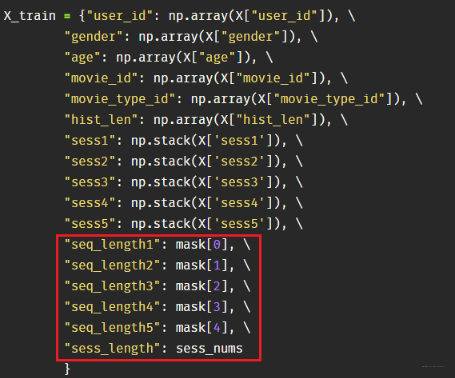
真实数据要和 Input 层接收进行对应好。
好了,关于数据处理就说这几个细节,感觉 mask 的那个处理非常需要注意。具体的看代码就可以啦。下面重头戏,剖析模型。
DSIN 模型全貌
有了 Deepctr 的这种代码风格,使得建立模型会从宏观上看起来非常清晰,简单说下逻辑, 先建立输入层,由于输入的特征有三大类 (离散,连续和变长离散),所以分别建立 Input 层,然后离散特征还得建立 embedding 层。下面三大类特征就有了不同的走向:
- 连续特征: 这类特征拼先拼接到一块,然后等待最后往 DNN 里面输入
- 普通离散特征: 这块从输入 -> embedding -> 拼接到一块,等待 DNN 里面输入
- 用户的会话特征:这块从输入 -> embedding -> 会话兴趣分割层 (
sess_interest_division) -> 会话兴趣提取层 (sess_interest_extractor) -> 会话兴趣交互层 (BiLSTM) -> 会话兴趣激活层 (AttentionPoolingLayer) -> 得到两个兴趣性特征
把上面的连续特征,离散特征和兴趣特征拼接起来,然后过 DNN 得到输出即可。就是这么个逻辑了,具体代码如下:
def DSIN(feature_columns, sess_feature_list, sess_max_count=5, bias_encoding=True, singlehead_emb_size=1,
         att_head_nums=8, dnn_hidden_units=(200, 80)):
    """
    建立DSIN网络
    :param feature_columns:  A list, 每个特征的封装 nametuple形式
    :param behavior_feature_list: A list, 行为特征名称
    :param sess_max_count: 会话的个数
    :param bias_encoding: 是否偏置编码
    :singlehead_emb_size: 每个头的注意力的维度,注意这个和头数的乘积必须等于输入的embedding的维度
    :att_head_nums:  头的个数
    :dnn_hidden_units: 这个是全连接网络的神经元个数
    """

    # 检查下embedding设置的是否合法,因为这里有了多头注意力机制之后,我们要保证我们的embedding维度 = att_head_nums * att_embedding_size
    hist_emb_size = sum(
        map(lambda fc: fc.embedding_dim, filter(lambda fc: fc.name in sess_feature_list, [feature for feature in feature_columns if not isinstance(feature, str)]))
    )
    if singlehead_emb_size * att_head_nums != hist_emb_size:
        raise ValueError(
            "hist_emb_size must equal to singlehead_emb_size * att_head_nums ,got %d != %d *%d" % (
                hist_emb_size, singlehead_emb_size, att_head_nums))

    # 建立输入层
    input_layer_dict = build_input_layers(feature_columns)
    # 将Input层转化为列表的形式作为model的输入
    input_layers = list(input_layer_dict.values())       # 各个输入层
    input_keys = list(input_layer_dict.keys())         # 各个列名
    user_sess_seq_len = [input_layer_dict['seq_length'+str(i+1)] for i in range(sess_max_count)]
    user_sess_len = input_layer_dict['sess_length']

    # 筛选出特征中的sparse_fra, dense_fea, varlen_fea
    sparse_feature_columns = list(filter(lambda x: isinstance(x, SparseFeat), feature_columns)) if feature_columns else []
    dense_feature_columns = list(filter(lambda x: isinstance(x, DenseFeat), feature_columns)) if feature_columns else []
    varlen_sparse_feature_columns = list(filter(lambda x: isinstance(x, VarLenSparseFeat), feature_columns)) if feature_columns else []

    # 获取dense
    dnn_dense_input = []
    for fc in dense_feature_columns:
        dnn_dense_input.append(input_layer_dict[fc.name])
    # 将所有的dense特征拼接
    dnn_dense_input = concat_input_list(dnn_dense_input)

    # 构建embedding词典
    embedding_layer_dict = build_embedding_layers(feature_columns, input_layer_dict)

    # 因为这里最终需要将embedding拼接后直接输入到全连接层(Dense)中, 所以需要Flatten
    dnn_sparse_embed_input = concat_embedding_list(sparse_feature_columns, input_layer_dict, embedding_layer_dict, flatten=True)
    # 将所有sparse特征的embedding进行拼接
    dnn_sparse_input = concat_input_list(dnn_sparse_embed_input)
    # dnn_dense_input和dnn_sparse_input这样就不用管了,等待后面的拼接就完事, 下面主要是会话行为兴趣的提取


    # 首先获取当前的行为特征(movie)的embedding,这里有可能有多个行为产生了行为序列,所以需要使用列表将其放在一起
    # 这个东西最后求局域Attention的时候使用,也就是选择与当前候选物品最相关的会话兴趣
    query_embed_list = embedding_lookup(sess_feature_list, input_layer_dict, embedding_layer_dict)
    query_emb = concat_input_list(query_embed_list)

    # 下面就是开始会话行为的处理了,四个层来: 会话分割层,会话兴趣提取层,会话兴趣交互层和局部Attention层,下面一一来做

    # 首先这里是找到会话行为中的特征列的输入层, 其实用input_layer_dict也行
    user_behavior_input_dict = {}
    for idx in range(sess_max_count):
        sess_input = OrderedDict()
        for i, feat in enumerate(sess_feature_list):  # 我这里只有一个movie_id
            sess_input[feat] = input_layer_dict["sess" + str(idx+1)]

        user_behavior_input_dict['sess'+str(idx+1)] = sess_input   # 这里其实是获取那五个会话的输入层

    # 会话兴趣分割层: 拿到每个会话里面各个商品的embedding,并且进行偏置编码,得到transformer的输入
    transformer_input = sess_interest_division(embedding_layer_dict, user_behavior_input_dict,
                                               sparse_feature_columns, sess_feature_list,
                                               sess_max_count, bias_encoding=bias_encoding)
    # 这个transformer_input是个列表,里面的每个元素代表一个会话,维度是(None, max_seq_len, embed_dim)

    # 会话兴趣提取层: 每个会话过transformer,从多个角度得到里面各个商品之间的相关性(交互)
    self_attention = Transformer(singlehead_emb_size, att_head_nums, dropout_rate=0, use_layer_norm=True,
                                 use_positional_encoding=(not bias_encoding), blinding=False)
    sess_fea = sess_interest_extractor(transformer_input, sess_max_count, self_attention, user_sess_seq_len)
    # 这里的输出sess_fea是个矩阵,维度(None, sess_max_cout, embed_dim), 这个东西后期要和当前的候选商品求Attention进行sess维度上的加权

    # 会话兴趣交互层  上面的transformer结果,过双向的LSTM
    lstm_output = BiLSTM(hist_emb_size, layers=2, res_layers=0, dropout_rate=0.2)(sess_fea)
    # 这个lstm_output是个矩阵,维度是(None, sess_max_count, hidden_units_num)

    # 会话兴趣激活层  这里就是计算两波注意力
    interest_attention = AttentionPoolingLayer(user_sess_len)([query_emb, sess_fea])
    lstm_attention = AttentionPoolingLayer(user_sess_len)([query_emb, lstm_output])
    # 上面这两个的维度分别是(None, embed_size), (None, hidden_units_num)  这里embed_size=hidden_units_num

    # 下面就是把dnn_sense_input, dnn_sparse_input, interest_attention, lstm_attention拼接起来
    deep_input = Concatenate(axis=-1)([dnn_dense_input, dnn_sparse_input, interest_attention, lstm_attention])

    # 全连接接网络, 获取最终的dnn_logits
    dnn_logits = get_dnn_logits(deep_input, activation='prelu')

    model = Model(input_layers, dnn_logits)

    # 所有变量需要初始化
    tf.compat.v1.keras.backend.get_session().run(tf.compat.v1.global_variables_initializer())

    return model
下面开始解释每块的细节实现。
会话兴趣分割层 (sess_interest_division)
这里面接收的输入是一个每个用户的会话列表, 比如上面那 5 个会话的时候,每个会话里面是有若干个商品的,当然还不仅仅是有商品 id,还有可能有类别 id 这种。 而这个函数干的事情就是遍历这 5 个会话,然后对于每个会话,要根据商品 id 拿到每个会话的商品 embedding (有类别 id 的话也会拿到类别 id 然后拼起来), 所以每个会话会得到一个 (None, seq_len, embed_dim) 的一个矩阵,而最后的输出就是 5 个会话的矩阵放到一个列表里返回来。也就是上面的 transformer_input , 作为 transformer 的输入。 这里面的一个细节,就是偏置编码。 如果需要偏置编码的话,要在这里面进行。偏置编码的过程
class BiasEncoding(Layer):
    """位置编码"""
    def __init__(self, sess_max_count, seed=1024):
        super(BiasEncoding, self).__init__()
        self.sess_max_count = sess_max_count
        self.seed = seed

    def build(self, input_shape):
        # 在该层创建一个可训练的权重  input_shape [None, sess_max_count, max_seq_len, embed_dim]
        if self.sess_max_count == 1:
            embed_size = input_shape[2]
            seq_len_max = input_shape[1]
        else:
            embed_size = input_shape[0][2]
            seq_len_max = input_shape[0][1]
        # 声明那三个位置偏置编码矩阵
        self.sess_bias_embedding = self.add_weight('sess_bias_encoding', shape=(self.sess_max_count, 1, 1),
                                                   initializer=tf.keras.initializers.TruncatedNormal(mean=0.0, stddev=0.0001, seed=self.seed))  # 截断产生正太随机数
        self.seq_bias_embedding = self.add_weight('seq_bias_encoding', shape=(1, seq_len_max, 1),
                                                  initializer=tf.keras.initializers.TruncatedNormal(mean=0.0, stddev=0.0001, seed=self.seed))
        self.embed_bias_embedding = self.add_weight('embed_beas_encoding', shape=(1, 1, embed_size),
                                                    initializer=tf.keras.initializers.TruncatedNormal(mean=0.0, stddev=0.0001, seed=self.seed))
        super(BiasEncoding, self).build(input_shape)

    def call(self, inputs, mask=None):
        """
        :param inputs:  A list 长度是会话数量,每个元素表示一个会话矩阵,维度是[None, max_seq_len, embed_dim]
        """
        bias_encoding_out = []
        for i in range(self.sess_max_count):
            bias_encoding_out.append(
                inputs[i] + self.embed_bias_embedding  + self.seq_bias_embedding + self.sess_bias_embedding[i]  # 这里会广播
            )
        return bias_encoding_out
这里的核心就是 build 里面的那三个偏置矩阵,对应论文里面的
会话兴趣提取层 (sess_interest_extractor)
这里面就是复现了大名鼎鼎的 Transformer 了, 这也是我第一次看 transformer 的代码,果真与之前的理论分析还是有很多不一样的点,下面得一一梳理一下,Transformer 是非常重要的。
首先是位置编码, 代码如下:
def positional_encoding(inputs, pos_embedding_trainable=True,scale=True):
    """
    inputs: (None, max_seq_len, embed_dim)
    """
    _, T, num_units = inputs.get_shape().as_list() # [None, max_seq_len, embed_dim]

    position_ind = tf.expand_dims(tf.range(T), 0)  # [1, max_seq_len]

    # First part of the PE function: sin and cos argument
    position_enc = np.array([
        [pos / np.power(1000, 2. * i / num_units) for i in range(num_units)] for pos in range(T)
    ])

    # Second part, apply the cosine to even columns and sin to odds.  # 这个操作秀
    position_enc[:, 0::2] = np.sin(position_enc[:, 0::2])  # dim 2i
    position_enc[:, 1::2] = np.cos(position_enc[:, 1::2])  # dim 2i+1

    # 转成张量
    if pos_embedding_trainable:
        lookup_table = K.variable(position_enc, dtype=tf.float32)

    outputs = tf.nn.embedding_lookup(lookup_table, position_ind)
    if scale:
        outputs = outputs * num_units ** 0.5
    return outputs + inputs
这一块的话没有啥好说的东西感觉,这个就是在按照论文里面的公式 sin, cos 变换, 这里面比较秀的操作感觉就是 dim2i 和 dim 2i+1 的赋值了。
接下来,LayerNormalization, 这个也是按照论文里面的公式实现的代码,求均值和方差的维度都是 embedding:
class LayerNormalization(Layer):
    def __init__(self, axis=-1, eps=1e-9, center=True, scale=True):
        super(LayerNormalization, self).__init__()
        self.axis = axis
        self.eps = eps
        self.center = center
        self.scale = scale
    def build(self, input_shape):
        """
        input_shape: [None, max_seq_len, singlehead_emb_dim*head_num]
        """
        self.gamma = self.add_weight(name='gamma', shape=input_shape[-1:],  # [1, max_seq_len, singlehead_emb_dim*head_num]
                                     initializer=tf.keras.initializers.Ones(), trainable=True)
        self.beta = self.add_weight(name='beta', shape=input_shape[-1:],
                                    initializer=tf.keras.initializers.Zeros(), trainable=True) # [1, max_seq_len, singlehead_emb_dim*head_num]
        super(LayerNormalization, self).build(input_shape)

    def call(self, inputs):
        """
           [None, max_seq_len, singlehead_emb_dim*head_num]
        """
        mean = K.mean(inputs, axis=self.axis, keepdims=True)  # embed_dim维度上求均值
        variance = K.mean(K.square(inputs-mean), axis=-1, keepdims=True)   # embed_dim维度求方差
        std = K.sqrt(variance + self.eps)
        outputs = (inputs - mean) / std

        if self.scale:
            outputs *= self.gamma
        if self.center:
            outputs += self.beta
        return outputs
下面就是伟大的 Transformer 网络,下面我先把整体代码放上来,然后解释一些和我之前见到过的一样的地方,也是通过看具体代码学习到的点:
class Transformer(Layer):
    """Transformer网络"""
    def __init__(self, singlehead_emb_size=1, att_head_nums=8, dropout_rate=0.0, use_positional_encoding=False,use_res=True,
                 use_feed_forword=True, use_layer_norm=False, blinding=False, seed=1024):
        super(Transformer, self).__init__()
        self.singlehead_emb_size = singlehead_emb_size
        self.att_head_nums = att_head_nums
        self.num_units = self.singlehead_emb_size * self.att_head_nums
        self.use_res = use_res
        self.use_feed_forword = use_feed_forword
        self.dropout_rate = dropout_rate
        self.use_positional_encoding = use_positional_encoding
        self.use_layer_norm = use_layer_norm
        self.blinding = blinding                   # 如果为True的话表明进行attention的时候未来的units都被屏蔽, 解码器的时候用
        self.seed = seed

    # 这里需要为该层自定义可训练的参数矩阵 WQ, WK, WV
    def build(self, input_shape):
        # input_shape: [None, max_seq_len, embed_dim]
        embedding_size= int(input_shape[0][-1])
        # 检查合法性
        if self.num_units != embedding_size:
            raise ValueError(
                "att_embedding_size * head_num must equal the last dimension size of inputs,got %d * %d != %d" % (
                self.singlehead_emb_size, att_head_nums, embedding_size))
        self.seq_len_max = int(input_shape[0][-2])
        # 定义三个矩阵
        self.W_Query = self.add_weight(name='query', shape=[embedding_size, self.singlehead_emb_size*self.att_head_nums],
                                       dtype=tf.float32,initializer=tf.keras.initializers.TruncatedNormal(seed=self.seed))
        self.W_Key = self.add_weight(name='key', shape=[embedding_size, self.singlehead_emb_size*self.att_head_nums],
                                       dtype=tf.float32,initializer=tf.keras.initializers.TruncatedNormal(seed=self.seed+1))
        self.W_Value = self.add_weight(name='value', shape=[embedding_size, self.singlehead_emb_size*self.att_head_nums],
                                       dtype=tf.float32,initializer=tf.keras.initializers.TruncatedNormal(seed=self.seed+2))
        # 用神经网络的话,加两层训练参数
        if self.use_feed_forword:
            self.fw1 = self.add_weight('fw1', shape=[self.num_units, 4 * self.num_units], dtype=tf.float32,
                                       initializer=tf.keras.initializers.glorot_uniform(seed=self.seed))
            self.fw2 = self.add_weight('fw2', shape=[4 * self.num_units, self.num_units], dtype=tf.float32,
                                       initializer=tf.keras.initializers.glorot_uniform(seed=self.seed+1))
        self.dropout = tf.keras.layers.Dropout(self.dropout_rate)
        self.ln = LayerNormalization()
        super(Transformer, self).build(input_shape)

    def call(self, inputs, mask=None, training=None):
        """
        :param inputs: [当前会话sessi, 当前会话sessi]  维度 (None, max_seq_len, embed_dim)
        :param mask: 当前会话mask  这是个1维数组, 维度是(None, ), 表示每个样本在当前会话里面的行为序列长度
        """
        # q和k其实是一样的矩阵
        queries, keys = inputs
        query_masks, key_masks = mask, mask

        # 这里需要对Q和K进行mask操作,
        # key masking目的是让key值的unit为0的key对应的attention score极小,这样加权计算value时相当于对结果不产生影响
        # Query Masking 要屏蔽的是被0所填充的内容。
        query_masks = tf.sequence_mask(query_masks, self.seq_len_max, dtype=tf.float32) # (None, 1, seq_len_max)
        key_masks = tf.sequence_mask(key_masks, self.seq_len_max, dtype=tf.float32)  # (None, 1, seq_len_max), 注意key_masks开始是(None,1)
        key_masks = key_masks[:, 0, :]     # 所以上面会多出个1维度来, 这里去掉才行,(None, seq_len_max)
        query_masks = query_masks[:, 0, :]   # 这个同理

        # 是否位置编码
        if self.use_positional_encoding:
            queries = positional_encoding(queries)
            keys = positional_encoding(queries)

        # tensordot 是矩阵乘,好处是当两个矩阵维度不同的时候,只要指定axes也可以乘
        # 这里表示的是queries的-1维度与W_Query的0维度相乘
        # (None, max_seq_len, embedding_size) * [embedding_size, singlehead_emb_size*head_num]
        querys = tf.tensordot(queries, self.W_Query, axes=(-1, 0)) # [None, max_seq_len_q, singlehead_emb_size*head_num]

        keys = tf.tensordot(keys, self.W_Key, axes=(-1, 0)) # [None, max_seq_len_k, singlehead_emb_size*head_num]
        values = tf.tensordot(keys, self.W_Value, axes=(-1, 0)) # [None, max_seq_len_k, singlehead_emb_size*head_num]

        # tf.split切分张量 这里从头那里切分成head_num个张量, 然后从0维拼接
        querys = tf.concat(tf.split(querys, self.att_head_nums, axis=2), axis=0)  # [head_num*None, max_seq_len_q, singlehead_emb_size]
        keys = tf.concat(tf.split(keys, self.att_head_nums, axis=2), axis=0) # [head_num*None, max_seq_len_k, singlehead_emb_size]
        values = tf.concat(tf.split(values, self.att_head_nums, axis=2), axis=0) # [head_num*None, max_seq_len_k, singlehead_emb_size]

        # Q*K   keys后两维转置然后再乘 [head_num*None, max_seq_len_q, max_seq_len_k]
        outputs = tf.matmul(querys, keys, transpose_b=True)
        outputs = outputs / (keys.get_shape().as_list()[-1] ** 0.5)

        # 从0维度上复制head_num次
        key_masks = tf.tile(key_masks, [self.att_head_nums, 1])  # [head_num*None, max_seq_len_k]
        key_masks = tf.tile(tf.expand_dims(key_masks, 1), [1, tf.shape(queries)[1], 1])  # [head_num*None, max_seq_len_q,max_seq_len_k]
        paddings = tf.ones_like(outputs) * (-2**32+1)

        outputs = tf.where(tf.equal(key_masks, 1), outputs, paddings)     # 被填充的部分赋予极小的权重

        #  标识是否屏蔽未来序列的信息(解码器self attention的时候不能看到自己之后的哪些信息)
        #  这里通过下三角矩阵的方式进行,依此表示预测第一个词,第二个词,第三个词...
        if self.blinding:
            diag_vals = tf.ones_like(outputs[0, :, :])  # (T_q, T_k)
            tril = tf.linalg.LinearOperatorLowerTriangular(diag_vals).to_dense()  # (T_q, T_k)   这是个下三角矩阵
            masks = tf.tile(tf.expand_dims(tril, 0), [tf.shape(outputs)[0], 1, 1])  # (h*N, T_q, T_k)

            paddings = tf.ones_like(masks) * (-2 ** 32 + 1)
            outputs = tf.where(tf.equal(masks, 0), paddings, outputs)  # (h*N, T_q, T_k)

        outputs -= tf.reduce_max(outputs, axis=-1, keepdims=True)
        outputs = tf.nn.softmax(outputs, axis=-1)     # 最后一个维度求softmax,换成权重

        query_masks = tf.tile(query_masks, [self.att_head_nums, 1])  # [head_num*None, max_seq_len_q]
        query_masks = tf.tile(tf.expand_dims(query_masks, -1), [1, 1, tf.shape(keys)[1]])  # [head_num*None, max_seq_len_q, max_seq_len_k]

        outputs *= query_masks

        # 权重矩阵过下dropout  [head_num*None, max_seq_len_q, max_seq_len_k]
        outputs = self.dropout(outputs, training=training)

        # weighted sum [head_num*None, max_seq_len_q, max_seq_len_k] * # [head_num*None, max_seq_len_k, singlehead_emb_size]
        result = tf.matmul(outputs, values)  # [head_num*None, max_seq_len_q, singlehead_emb_size]
        # 换回去了
        result = tf.concat(tf.split(result, self.att_head_nums, axis=0), axis=2)  # [None, max_seq_len_q, head_num*singlehead_emb_size]

        if self.use_res:   # 残差连接
            result += queries
        if self.use_layer_norm:
            result = self.ln(result)
        if self.use_feed_forword: # [None, max_seq_len_q, head_num*singlehead_emb_size] 与 [num_units, self.num_units]
            fw1 = tf.nn.relu(tf.tensordot(result, self.fw1, axes=[-1, 0])) # [None, max_seq_len_q, 4*num_units]
            fw1 = self.dropout(fw1, training=training)
            fw2 = tf.tensordot(fw1, self.fw2, axes=[-1, 0])  # [None, max_seq_len_q, num_units]  这个num_units其实就等于head_num*singlehead_emb_size

            if self.use_res:
                result += fw2
            if self.use_layer_norm:
                result = self.ln(result)

        return tf.reduce_mean(result, axis=1, keepdims=True)  # [None, 1, head_num*singleh]
这里面的整体逻辑, 首先在 build 里面会构建 3 个矩阵 WQ, WK, WV ,在这里定义依然是为了这些参数可训练, 而出乎我意料的是残差网络的参数 w 也是这里定义, 之前还以为这个是单独写出来,后面看了前向传播的逻辑时候明白了。
前向传播的逻辑和我之前画的图上差不多,不一样的细节是这里的具体实现上, 就是这里的把多个头分开,采用堆叠的方式进行计算 (堆叠到第一个维度上去了)。这个是我之前忽略的一个问题, 只有这样才能使得每个头与每个头之间的自注意力运算是独立不影响的。如果不这么做的话,最后得到的结果会含有当前单词在这个头和另一个单词在另一个头上的关联,这是不合理的。这是看了源码之后才发现的细节。
另外就是 mask 操作这里,Q 和 K 都需要进行 mask 操作,因为我们接受的输入序列是经过填充的,这里必须通过指明长度在具体计算的时候进行遮盖,否则 softmax 那里算的时候会有影响,因为 e 的 0 次方是 1,所以这里需要找到序列里面填充的那些地方,给他一个超级大的负数,这样 e 的负无穷接近 0,才能没有影响。但之前不知道这里的细节,这次看发现是 Q 和 K 都进行 mask 操作,且目的还不一样。
第三个细节,就是对未来序列的屏蔽,这个在这里是用不到的,这个是 Transformer 的解码器用的一个操作,就是在解码的时候,我们不能让当前的序列看到自己之后的信息。这里也需要进行 mask 遮盖住后面的。而具体实现,竟然使用了一个下三角矩阵, 这个东西的感觉是这样:
解码的时候,只能看到自己及以前的相关性,然后加权,这个学到了哈哈。
transformer 这里接收的是会话兴趣分割层传下来的兴趣列表,返回的是个矩阵,维度是 (None, sess_nums, embed_dim) , 因为这里每个会话都要过 Transformer, 输入的维度是 (None, seq_len, embed_dim), 而经过 transformer 之后,本来输出的维度也是这个,但是最后返回的时候在 seq_len 的维度上求了个平均。所以每个会话得到的输出是 (None, 1, embed_dim), 相当于兴趣综合了下。而 5 个会话,就会得到 5 个这样的结果,然后再会话维度上拼接,就是上面的这个矩阵结果了,这个东西作为双向 LSTM 的输入。
会话兴趣交互层 (BiLSTM)
这里主要是值得记录下多层双向 LSTM 的实现过程, 用下面的这种方式非常的灵活:
class BiLSTM(Layer):
    def __init__(self, units, layers=2, res_layers=0, dropout_rate=0.2, merge_mode='ave'):
        super(BiLSTM, self).__init__()
        self.units = units
        self.layers = layers
        self.res_layers = res_layers
        self.dropout_rate = dropout_rate
        self.merge_mode = merge_mode

    # 这里要构建正向的LSTM和反向的LSTM, 因为我们是要两者的计算结果最后加和,所以这里需要分别计算
    def build(self, input_shape):
        """
        input_shape: (None, sess_max_count, embed_dim)
        """
        self.fw_lstm = []
        self.bw_lstm = []
        for _ in range(self.layers):
            self.fw_lstm.append(
                LSTM(self.units, dropout=self.dropout_rate, bias_initializer='ones', return_sequences=True, unroll=True)
            )
            # go_backwards 如果为真,则反向处理输入序列并返回相反的序列
            # unroll 布尔(默认错误)。如果为真,则网络将展开,否则使用符号循环。展开可以提高RNN的速度,尽管它往往会占用更多的内存。展开只适用于较短的序列。
            self.bw_lstm.append(
                LSTM(self.units, dropout=self.dropout_rate, bias_initializer='ones', return_sequences=True, go_backwards=True, unroll=True)
            )
        super(BiLSTM, self).build(input_shape)

    def call(self, inputs):

        input_fw = inputs
        input_bw = inputs
        for i in range(self.layers):
            output_fw = self.fw_lstm[i](input_fw)
            output_bw = self.bw_lstm[i](input_bw)
            output_bw = Lambda(lambda x: K.reverse(x, 1), mask=lambda inputs, mask:mask)(output_bw)

            if i >= self.layers - self.res_layers:
                output_fw += input_fw
                output_bw += input_bw

            input_fw = output_fw
            input_bw = output_bw

        if self.merge_mode == "fw":
            output = output_fw
        elif self.merge_mode == "bw":
            output = output_bw
        elif self.merge_mode == 'concat':
            output = K.concatenate([output_fw, output_bw])
        elif self.merge_mode == 'sum':
            output = output_fw + output_bw
        elif self.merge_mode == 'ave':
            output = (output_fw + output_bw) / 2
        elif self.merge_mode == 'mul':
            output = output_fw * output_bw
        elif self.merge_mode is None:
            output = [output_fw, output_bw]

        return output
这里这个操作是比较骚的,以后建立双向 LSTM 就用这个模板了,具体也不用解释,并且这里之所以说灵活,是因为最后前向 LSTM 的结果和反向 LSTM 的结果都能单独的拿到,且可以任意的两者运算。 我记得 Keras 里面应该是也有直接的函数实现双向 LSTM 的,但依然感觉不如这种灵活。 这个层数自己定,单元自己定看,最后结果形式自己定,太帅了简直。 关于 LSTM,可以看官方文档
这个的输入是 (None, sess_nums, embed_dim) , 输出是 (None, sess_nums, hidden_units_num) 。
会话兴趣局部激活
这里就是局部 Attention 的操作了,这个在这里就不解释了,和之前的 DIEN,DIN 的操作就一样了, 代码也不放在这里了,剩下的代码都看后面的 GitHub 链接吧, 这里我只记录下我觉得后面做别的项目会有用的代码哈哈。
总结
DSIN 的核心创新点就是把用户的历史行为按照时间间隔进行切分,以会话为单位进行学习, 而学习的方式首先是会话之内的行为自学习,然后是会话之间的交互学习,最后是与当前候选商品相关的兴趣演进,总体上还是挺清晰的。
具体的实际使用场景依然是有丰富的用户历史行为序列才可以,而会话之间的划分间隔,也得依据具体业务场景。 具体的使用可以调 deepctr 的包。
参考资料: